45. Optimal Growth II: Accelerating the Code with Numba #

Contents

Optimal Growth II: Accelerating the Code with Numba

In addition to what’s in Anaconda, this lecture will need the following libraries:

!pip install quantecon

45.1. Overview #

Previously, we studied a stochastic optimal growth model with one representative agent.

We solved the model using dynamic programming.

In writing our code, we focused on clarity and flexibility.

These are important, but there’s often a trade-off between flexibility and speed.

The reason is that, when code is less flexible, we can exploit structure more easily.

(This is true about algorithms and mathematical problems more generally: more specific problems have more structure, which, with some thought, can be exploited for better results.)

So, in this lecture, we are going to accept less flexibility while gaining speed, using just-in-time (JIT) compilation to accelerate our code.

Let’s start with some imports:

import matplotlib.pyplot as plt
import numpy as np
from numba import jit, njit
from quantecon.optimize.scalar_maximization import brent_max

The function brent_max is also designed for embedding in JIT-compiled code.

These are alternatives to similar functions in SciPy (which, unfortunately, are not JIT-aware).

45.2. The Model #

The model is the same as discussed in our previous lecture on optimal growth.

We will start with log utility:

\[ u(c) = \ln(c) \]

We continue to assume that

\(f(k) = k^{\alpha}\)
\(\phi\) is the distribution of \(\xi := \exp(\mu + s \zeta)\) when \(\zeta\) is standard normal

We will once again use value function iteration to solve the model.

In particular, the algorithm is unchanged, and the only difference is in the implementation itself.

As before, we will be able to compare with the true solutions

def v_star(y, α, β, μ):
    """
    True value function
    """
    c1 = np.log(1 - α * β) / (1 - β)
    c2 = (μ + α * np.log(α * β)) / (1 - α)
    c3 = 1 / (1 - β)
    c4 = 1 / (1 - α * β)
    return c1 + c2 * (c3 - c4) + c4 * np.log(y)

def σ_star(y, α, β):
    """
    True optimal policy
    """
    return (1 - α * β) * y

45.3. Computation #

We will again store the primitives of the optimal growth model in a class.

But now we are going to use Numba’s @jitclass decorator to target our class for JIT compilation.

Because we are going to use Numba to compile our class, we need to specify the data types.

You will see this as a list called opt_growth_data above our class.

Unlike in the previous lecture, we hardwire the production and utility specifications into the class.

This is where we sacrifice flexibility in order to gain more speed.

from numba import float64
from numba.experimental import jitclass

opt_growth_data = [
    ('α', float64),          # Production parameter
    ('β', float64),          # Discount factor
    ('μ', float64),          # Shock location parameter
    ('s', float64),          # Shock scale parameter
    ('grid', float64[:]),    # Grid (array)
    ('shocks', float64[:])   # Shock draws (array)
]

@jitclass(opt_growth_data)
class OptimalGrowthModel:

    def __init__(self,
                α=0.4,
                β=0.96,
                μ=0,
                s=0.1,
                grid_max=4,
                grid_size=120,
                shock_size=250,
                seed=1234):

        self.α, self.β, self.μ, self.s = α, β, μ, s

        # Set up grid
        self.grid = np.linspace(1e-5, grid_max, grid_size)

        # Store shocks (with a seed, so results are reproducible)
        np.random.seed(seed)
        self.shocks = np.exp(μ + s * np.random.randn(shock_size))


    def f(self, k):
        "The production function"
        return k**self.α


    def u(self, c):
        "The utility function"
        return np.log(c)

    def f_prime(self, k):
        "Derivative of f"
        return self.α * (k**(self.α - 1))


    def u_prime(self, c):
        "Derivative of u"
        return 1/c

    def u_prime_inv(self, c):
        "Inverse of u'"
        return 1/c

The class includes some methods such as u_prime that we do not need now but will use in later lectures.

45.3.1. The Bellman Operator#

We will use JIT compilation to accelerate the Bellman operator.

First, here’s a function that returns the value of a particular consumption choice c, given state y, as per the Bellman equation (44.9).

@njit
def state_action_value(c, y, v_array, og):
    """
    Right hand side of the Bellman equation.

     * c is consumption
     * y is income
     * og is an instance of OptimalGrowthModel
     * v_array represents a guess of the value function on the grid

    """

    u, f, β, shocks = og.u, og.f, og.β, og.shocks

    v = lambda x: np.interp(x, og.grid, v_array)

    return u(c) + β * np.mean(v(f(y - c) * shocks))

Now we can implement the Bellman operator, which maximizes the right hand side of the Bellman equation:

@jit(nopython=True)
def T(v, og):
    """
    The Bellman operator.

     * og is an instance of OptimalGrowthModel
     * v is an array representing a guess of the value function

    """

    v_new = np.empty_like(v)
    v_greedy = np.empty_like(v)

    for i in range(len(og.grid)):
        y = og.grid[i]

        # Maximize RHS of Bellman equation at state y
        result = brent_max(state_action_value, 1e-10, y, args=(y, v, og))
        v_greedy[i], v_new[i] = result[0], result[1]

    return v_greedy, v_new

We use the solve_model function to perform iteration until convergence.

def solve_model(og,
                tol=1e-4,
                max_iter=1000,
                verbose=True,
                print_skip=25):
    """
    Solve model by iterating with the Bellman operator.

    """

    # Set up loop
    v = og.u(og.grid)  # Initial condition
    i = 0
    error = tol + 1

    while i < max_iter and error > tol:
        v_greedy, v_new = T(v, og)
        error = np.max(np.abs(v - v_new))
        i += 1
        if verbose and i % print_skip == 0:
            print(f"Error at iteration {i} is {error}.")
        v = v_new

    if error > tol:
        print("Failed to converge!")
    elif verbose:
        print(f"\nConverged in {i} iterations.")

    return v_greedy, v_new

Let’s compute the approximate solution at the default parameters.

First we create an instance:

og = OptimalGrowthModel()

Now we call solve_model, using the %%time magic to check how long it takes.

%%time
v_greedy, v_solution = solve_model(og)

Error at iteration 25 is 0.41372668361362486.

Error at iteration 50 is 0.14767653072603082.

Error at iteration 75 is 0.053221715530327174.

Error at iteration 100 is 0.019180931418517844.

Error at iteration 125 is 0.0069127447095276295.

Error at iteration 150 is 0.0024913304978255724.

Error at iteration 175 is 0.0008978673320818586.

Error at iteration 200 is 0.0003235884387500221.

Error at iteration 225 is 0.00011662021095659725.

Converged in 229 iterations.
CPU times: user 5.73 s, sys: 415 ms, total: 6.14 s
Wall time: 6.13 s

You will notice that this is much faster than our original implementation.

Here is a plot of the resulting policy, compared with the true policy:

fig, ax = plt.subplots()

ax.plot(og.grid, v_greedy, lw=2,
        alpha=0.8, label='approximate policy function')

ax.plot(og.grid, σ_star(og.grid, og.α, og.β), 'k--',
        lw=2, alpha=0.8, label='true policy function')

ax.legend()
plt.show()

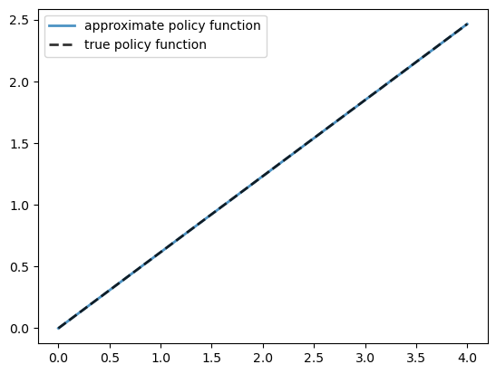
_images/a8d581d09c7a1e989e4dc1bc1e5c1fcd6468897829b987c59642d0fb864c0af0.png

Again, the fit is excellent — this is as expected since we have not changed the algorithm.

The maximal absolute deviation between the two policies is

np.max(np.abs(v_greedy - σ_star(og.grid, og.α, og.β)))

0.0010480495434626036

45.4. Exercises #

Exercise 45.1

Time how long it takes to iterate with the Bellman operator 20 times, starting from initial condition \(v(y) = u(y)\).

Use the default parameterization.

Solution to Exercise 45.1

Let’s set up the initial condition.

v = og.u(og.grid)

Here’s the timing:

%%time

for i in range(20):
    v_greedy, v_new = T(v, og)
    v = v_new

CPU times: user 209 ms, sys: 0 ns, total: 209 ms
Wall time: 209 ms

Compared with our timing for the non-compiled version of value function iteration, the JIT-compiled code is usually an order of magnitude faster.

Exercise 45.2

Modify the optimal growth model to use the CRRA utility specification.

\[ u(c) = \frac{c^{1 - \gamma} } {1 - \gamma} \]

Set γ = 1.5 as the default value and maintaining other specifications.

(Note that jitclass currently does not support inheritance, so you will have to copy the class and change the relevant parameters and methods.)

Compute an estimate of the optimal policy, plot it and compare visually with the same plot from the analogous exercise in the first optimal growth lecture.

Compare execution time as well.

Solution to Exercise 45.2

Here’s our CRRA version of OptimalGrowthModel:

from numba import float64
from numba.experimental import jitclass

opt_growth_data = [
    ('α', float64),          # Production parameter
    ('β', float64),          # Discount factor
    ('μ', float64),          # Shock location parameter
    ('γ', float64),          # Preference parameter
    ('s', float64),          # Shock scale parameter
    ('grid', float64[:]),    # Grid (array)
    ('shocks', float64[:])   # Shock draws (array)
]

@jitclass(opt_growth_data)
class OptimalGrowthModel_CRRA:

    def __init__(self,
                α=0.4,
                β=0.96,
                μ=0,
                s=0.1,
                γ=1.5,
                grid_max=4,
                grid_size=120,
                shock_size=250,
                seed=1234):

        self.α, self.β, self.γ, self.μ, self.s = α, β, γ, μ, s

        # Set up grid
        self.grid = np.linspace(1e-5, grid_max, grid_size)

        # Store shocks (with a seed, so results are reproducible)
        np.random.seed(seed)
        self.shocks = np.exp(μ + s * np.random.randn(shock_size))


    def f(self, k):
        "The production function."
        return k**self.α

    def u(self, c):
        "The utility function."
        return c**(1 - self.γ) / (1 - self.γ)

    def f_prime(self, k):
        "Derivative of f."
        return self.α * (k**(self.α - 1))

    def u_prime(self, c):
        "Derivative of u."
        return c**(-self.γ)

    def u_prime_inv(c):
        return c**(-1 / self.γ)

Let’s create an instance:

og_crra = OptimalGrowthModel_CRRA()

Now we call solve_model, using the %%time magic to check how long it takes.

%%time
v_greedy, v_solution = solve_model(og_crra)

Error at iteration 25 is 1.6201897527239453.

Error at iteration 50 is 0.459106047057503.

Error at iteration 75 is 0.16542352216310974.

Error at iteration 100 is 0.05961808343499797.

Error at iteration 125 is 0.02148616153202454.

Error at iteration 150 is 0.007743542074422294.

Error at iteration 175 is 0.0027907471408212814.

Error at iteration 200 is 0.0010057761073767324.

Error at iteration 225 is 0.0003624784085332067.

Error at iteration 250 is 0.00013063602807505958.

Converged in 257 iterations.
CPU times: user 4.61 s, sys: 107 ms, total: 4.71 s
Wall time: 4.71 s

Here is a plot of the resulting policy:

fig, ax = plt.subplots()

ax.plot(og.grid, v_greedy, lw=2,
        alpha=0.6, label='Approximate value function')

ax.legend(loc='lower right')
plt.show()

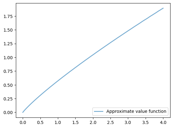
_images/937dc6e2065f21e70a77a826916e6a710765396551ebfbdad3f4bd7f4245e6a9.png

This matches the solution that we obtained in our non-jitted code, in the exercises.

Execution time is an order of magnitude faster.

Exercise 45.3

In this exercise we return to the original log utility specification.

Once an optimal consumption policy \(\sigma\) is given, income follows

\[ y_{t+1} = f(y_t - \sigma(y_t)) \xi_{t+1} \]

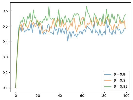
The next figure shows a simulation of 100 elements of this sequence for three different discount factors (and hence three different policies).

In each sequence, the initial condition is \(y_0 = 0.1\).

The discount factors are discount_factors = (0.8, 0.9, 0.98).

We have also dialed down the shocks a bit with s = 0.05.

Otherwise, the parameters and primitives are the same as the log-linear model discussed earlier in the lecture.

Notice that more patient agents typically have higher wealth.

Replicate the figure modulo randomness.

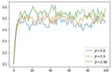
Solution to Exercise 45.3

Here’s one solution:

def simulate_og(σ_func, og, y0=0.1, ts_length=100):
    '''
    Compute a time series given consumption policy σ.
    '''
    y = np.empty(ts_length)
    ξ = np.random.randn(ts_length-1)
    y[0] = y0
    for t in range(ts_length-1):
        y[t+1] = (y[t] - σ_func(y[t]))**og.α * np.exp(og.μ + og.s * ξ[t])
    return y

fig, ax = plt.subplots()

for β in (0.8, 0.9, 0.98):

    og = OptimalGrowthModel(β=β, s=0.05)

    v_greedy, v_solution = solve_model(og, verbose=False)

    # Define an optimal policy function
    σ_func = lambda x: np.interp(x, og.grid, v_greedy)
    y = simulate_og(σ_func, og)
    ax.plot(y, lw=2, alpha=0.6, label=rf'$\beta = {β}$')

ax.legend(loc='lower right')
plt.show()

_images/8bd0f0d632f17b356c4bd747ed3dcaf59653cb51e0ad66f6bc70d509fc86cd89.png

45. Optimal Growth II: Accelerating the Code with Numba#

45.1. Overview#

45.2. The Model#

45.3. Computation#

45.3.1. The Bellman Operator#

45.4. Exercises#

45. Optimal Growth II: Accelerating the Code with Numba #

45.1. Overview #

45.2. The Model #

45.3. Computation #

45.4. Exercises #