55. Cake Eating I: Introduction to Optimal Saving#
55.1. Overview#
In this lecture we introduce a simple “cake eating” problem.
The intertemporal problem is: how much to enjoy today and how much to leave for the future?
Although the topic sounds trivial, this kind of trade-off between current and future utility is at the heart of many savings and consumption problems.
Once we master the ideas in this simple environment, we will apply them to progressively more challenging—and useful—problems.
The main tool we will use to solve the cake eating problem is dynamic programming.
Readers might find it helpful to review the following lectures before reading this one:
In what follows, we require the following imports:
import matplotlib.pyplot as plt
import numpy as np
55.2. The model#
We consider an infinite time horizon \(t=0, 1, 2, 3..\)
At \(t=0\) the agent is given a complete cake with size \(\bar x\).
Let \(x_t\) denote the size of the cake at the beginning of each period, so that, in particular, \(x_0=\bar x\).
We choose how much of the cake to eat in any given period \(t\).
After choosing to consume \(c_t\) of the cake in period \(t\) there is
left in period \(t+1\).
Consuming quantity \(c\) of the cake gives current utility \(u(c)\).
We adopt the CRRA utility function
In Python this is
def u(c, γ):

    return c**(1 - γ) / (1 - γ)
Future cake consumption utility is discounted according to \(\beta\in(0, 1)\).
In particular, consumption of \(c\) units \(t\) periods hence has present value \(\beta^t u(c)\)
The agent’s problem can be written as
subject to
for all \(t\).
A consumption path \(\{c_t\}\) satisfying (55.3) where \(x_0 = \bar x\) is called feasible.
In this problem, the following terminology is standard:
\(x_t\) is called the state variable
\(c_t\) is called the control variable or the action
\(\beta\) and \(\gamma\) are parameters
55.2.1. Trade-off#
The key trade-off in the cake-eating problem is this:
Delaying consumption is costly because of the discount factor.
But delaying some consumption is also attractive because \(u\) is concave.
The concavity of \(u\) implies that the consumer gains value from consumption smoothing, which means spreading consumption out over time.
This is because concavity implies diminishing marginal utility—a progressively smaller gain in utility for each additional spoonful of cake consumed within one period.
55.2.2. Intuition#
The reasoning given above suggests that the discount factor \(\beta\) and the curvature parameter \(\gamma\) will play a key role in determining the rate of consumption.
Here’s an educated guess as to what impact these parameters will have.
First, higher \(\beta\) implies less discounting, and hence the agent is more patient, which should reduce the rate of consumption.
Second, higher \(\gamma\) implies that marginal utility \(u'(c) = c^{-\gamma}\) falls faster with \(c\).
This suggests more smoothing, and hence a lower rate of consumption.
In summary, we expect the rate of consumption to be decreasing in both parameters.
Let’s see if this is true.
55.3. The value function#
The first step of our dynamic programming treatment is to obtain the Bellman equation.
The next step is to use it to calculate the solution.
55.3.1. The Bellman equation#
To this end, we let \(v(x)\) be maximum lifetime utility attainable from the current time when \(x\) units of cake are left.
That is,
where the maximization is over all paths \(\{ c_t \}\) that are feasible from \(x_0 = x\).
At this point, we do not have an expression for \(v\), but we can still make inferences about it.
For example, as was the case with the McCall model, the value function will satisfy a version of the Bellman equation.
In the present case, this equation states that \(v\) satisfies
The intuition here is essentially the same it was for the McCall model.
Choosing \(c\) optimally means trading off current vs future rewards.
Current rewards from choice \(c\) are just \(u(c)\).
Future rewards given current cake size \(x\), measured from next period and assuming optimal behavior, are \(v(x-c)\).
These are the two terms on the right hand side of (55.5), after suitable discounting.
If \(c\) is chosen optimally using this trade off strategy, then we obtain maximal lifetime rewards from our current state \(x\).
Hence, \(v(x)\) equals the right hand side of (55.5), as claimed.
55.3.2. An analytical solution#
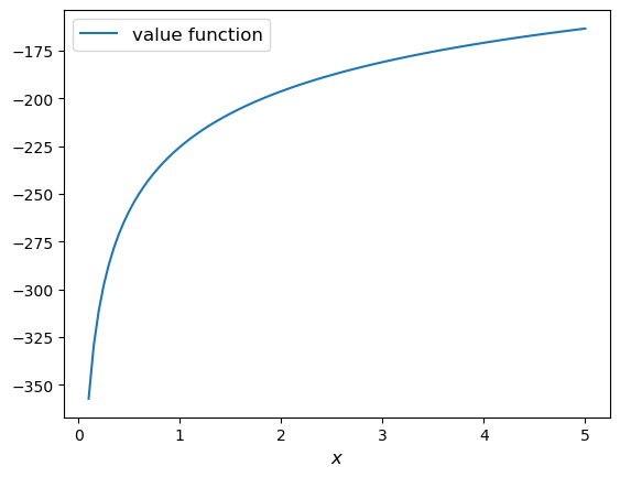
It has been shown that, with \(u\) as the CRRA utility function in (55.1), the function
solves the Bellman equation and hence is equal to the value function.
You are asked to confirm that this is true in the exercises below.
The solution (55.6) depends heavily on the CRRA utility function.
In fact, if we move away from CRRA utility, usually there is no analytical solution at all.
In other words, beyond CRRA utility, we know that the value function still satisfies the Bellman equation, but we do not have a way of writing it explicitly, as a function of the state variable and the parameters.
We will deal with that situation numerically when the time comes.
Here is a Python representation of the value function:
def v_star(x, β, γ):

    return (1 - β**(1 / γ))**(-γ) * u(x, γ)
And here’s a figure showing the function for fixed parameters:
β, γ = 0.95, 1.2
x_grid = np.linspace(0.1, 5, 100)

fig, ax = plt.subplots()

ax.plot(x_grid, v_star(x_grid, β, γ), label='value function')

ax.set_xlabel('$x$', fontsize=12)
ax.legend(fontsize=12)

plt.show()
55.4. The optimal policy#
Now that we have the value function, it is straightforward to calculate the optimal action at each state.
We should choose consumption to maximize the right hand side of the Bellman equation (55.5).
We can think of this optimal choice as a function of the state \(x\), in which case we call it the optimal policy.
We denote the optimal policy by \(\sigma^*\), so that
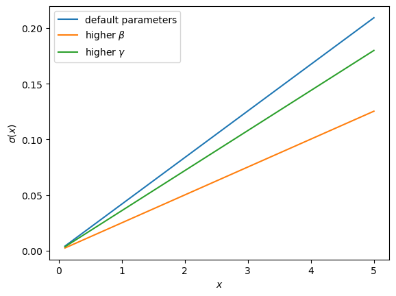
If we plug the analytical expression (55.6) for the value function into the right hand side and compute the optimum, we find that
Now let’s recall our intuition on the impact of parameters.
We guessed that the consumption rate would be decreasing in both parameters.
This is in fact the case, as can be seen from (55.7).
Here’s some plots that illustrate.
def c_star(x, β, γ):

    return (1 - β ** (1/γ)) * x
Continuing with the values for \(\beta\) and \(\gamma\) used above, the plot is
fig, ax = plt.subplots()
ax.plot(x_grid, c_star(x_grid, β, γ), label='default parameters')
ax.plot(x_grid, c_star(x_grid, β + 0.02, γ), label=r'higher $\beta$')
ax.plot(x_grid, c_star(x_grid, β, γ + 0.2), label=r'higher $\gamma$')
ax.set_ylabel(r'$\sigma(x)$')
ax.set_xlabel('$x$')
ax.legend()

plt.show()
55.5. The Euler equation#
In the discussion above we have provided a complete solution to the cake eating problem in the case of CRRA utility.
There is in fact another way to solve for the optimal policy, based on the so-called Euler equation.
Although we already have a complete solution, now is a good time to study the Euler equation.
This is because, for more difficult problems, this equation provides key insights that are hard to obtain by other methods.
55.5.1. Statement and implications#
The Euler equation for the present problem can be stated as
This is necessary condition for the optimal path.
It says that, along the optimal path, marginal rewards are equalized across time, after appropriate discounting.
This makes sense: optimality is obtained by smoothing consumption up to the point where no marginal gains remain.
We can also state the Euler equation in terms of the policy function.
A feasible consumption policy is a map \(x \mapsto \sigma(x)\) satisfying \(0 \leq \sigma(x) \leq x\).
The last restriction says that we cannot consume more than the remaining quantity of cake.
A feasible consumption policy \(\sigma\) is said to satisfy the Euler equation if, for all \(x > 0\),
Evidently (55.9) is just the policy equivalent of (55.8).
It turns out that a feasible policy is optimal if and only if it satisfies the Euler equation.
In the exercises, you are asked to verify that the optimal policy (55.7) does indeed satisfy this functional equation.
Note
A functional equation is an equation where the unknown object is a function.
For a proof of sufficiency of the Euler equation in a very general setting, see proposition 2.2 of [Ma et al., 2020].
The following arguments focus on necessity, explaining why an optimal path or policy should satisfy the Euler equation.
55.5.2. Derivation I: a perturbation approach#
Let’s write \(c\) as a shorthand for consumption path \(\{c_t\}_{t=0}^\infty\).
The overall cake-eating maximization problem can be written as
and \(F\) is the set of feasible consumption paths.
We know that differentiable functions have a zero gradient at a maximizer.
So the optimal path \(c^* := \{c^*_t\}_{t=0}^\infty\) must satisfy \(U'(c^*) = 0\).
Note
If you want to know exactly how the derivative \(U'(c^*)\) is defined, given that the argument \(c^*\) is a vector of infinite length, you can start by learning about Gateaux derivatives. However, such knowledge is not assumed in what follows.
In other words, the rate of change in \(U\) must be zero for any infinitesimally small (and feasible) perturbation away from the optimal path.
So consider a feasible perturbation that reduces consumption at time \(t\) to \(c^*_t - h\) and increases it in the next period to \(c^*_{t+1} + h\).
Consumption does not change in any other period.
We call this perturbed path \(c^h\).
By the preceding argument about zero gradients, we have
Recalling that consumption only changes at \(t\) and \(t+1\), this becomes
After rearranging, the same expression can be written as
or, taking the limit,
This is just the Euler equation.
55.5.3. Derivation II: using the Bellman equation#
Another way to derive the Euler equation is to use the Bellman equation (55.5).
Taking the derivative on the right hand side of the Bellman equation with respect to \(c\) and setting it to zero, we get
To obtain \(v^{\prime}(x - c)\), we set \(g(c,x) = u(c) + \beta v(x - c)\), so that, at the optimal choice of consumption,
Differentiating both sides while acknowledging that the maximizing consumption will depend on \(x\), we get
When \(g(c,x)\) is maximized at \(c\), we have \(\frac{\partial }{\partial c} g(c,x) = 0\).
Hence the derivative simplifies to
(This argument is an example of the Envelope Theorem.)
But now an application of (55.10) gives
Thus, the derivative of the value function is equal to marginal utility.
Combining this fact with (55.12) recovers the Euler equation.
55.6. Exercises#
Exercise 55.1
How does one obtain the expressions for the value function and optimal policy given in (55.6) and (55.7) respectively?
The first step is to make a guess of the functional form for the consumption policy.
So suppose that we do not know the solutions and start with a guess that the optimal policy is linear.
In other words, we conjecture that there exists a positive \(\theta\) such that setting \(c_t^*=\theta x_t\) for all \(t\) produces an optimal path.
Starting from this conjecture, try to obtain the solutions (55.6) and (55.7).
In doing so, you will need to use the definition of the value function and the Bellman equation.
Solution to Exercise 55.1
We start with the conjecture \(c_t^*=\theta x_t\), which leads to a path for the state variable (cake size) given by
Then \(x_t = x_{0}(1-\theta)^t\) and hence
From the Bellman equation, then,
From the first order condition, we obtain
or
With \(c = \theta x\) we get
Some rearrangement produces
This confirms our earlier expression for the optimal policy:
Substituting \(\theta\) into the value function above gives
Rearranging gives
Our claims are now verified.